Example using HBV model in eWaterCycle
1 In:
# general python
import warnings
warnings.filterwarnings("ignore", category=UserWarning)

import numpy as np
from pathlib import Path
import pandas as pd
import matplotlib.pyplot as plt
2 In:
# general eWC
import ewatercycle
import ewatercycle.models
import ewatercycle.forcing
Install required plugin with pip:
pip install ewatercycle-HBV
set up paths
3 In:
path = Path.cwd()
forcing_path = path / "Forcing"
forcing_path.mkdir(exist_ok=True)
add parameter info
Array of initial storage terms - we keep these constant for now: Si, Su, Sf, Ss
4 In:
s_0 = np.array([0, 100, 0, 5, 0])
Array of parameters min/max bounds as a reference: Imax, Ce, Sumax, beta, Pmax, T_lag, Kf, Ks
5 In:
p_min_initial= np.array([0,   0.2,  40,    .5,   .001,   1,     .01,  .0001, 6])
p_max_initial = np.array([8,    1,  800,   4,    .3,     10,    .1,   .01, 0.1])
p_names = ["$I_{max}$",  "$C_e$",  "$Su_{max}$", "β",  "$P_{max}$",  "$T_{lag}$",   "$K_f$",   "$K_s$", "FM"]
S_names = ["Interception storage", "Unsaturated Rootzone Storage", "Fastflow storage", "Groundwater storage", "Snowpack storage"]
param_names = ["Imax","Ce",  "Sumax", "Beta",  "Pmax",  "Tlag",   "Kf",   "Ks", "FM"]
stor_names = ["Si", "Su", "Sf", "Ss", "Sp"]
Set initial as mean of max,min
6 In:
par_0 = (p_min_initial + p_max_initial)/2
Specify start and end date
7 In:
experiment_start_date = "1997-08-01T00:00:00Z"
experiment_end_date = "2000-08-31T00:00:00Z"
HRU_id = 1620500
alpha = 1.2626
Forcing
8 In:
from ewatercycle_HBV.forcing import HBVForcing
we use camels forcing as an example, which is fully integrated Newman, 2014. The seperate text file is hosted here for easy access without having to download the whole dataset (13gb).
9 In:
camels_forcing = HBVForcing(start_time = experiment_start_date,
                          end_time = experiment_end_date,
                          directory = forcing_path,
                          camels_file = f'0{HRU_id}_lump_cida_forcing_leap.txt',
                          alpha= alpha
                          )
Setting up the model
10 In:
from ewatercycle.models import HBV
11 In:
model = HBV(forcing=camels_forcing)
12 In:
config_file, _ = model.setup(
            parameters=','.join([str(p) for p in par_0]),
    initial_storage=','.join([str(s) for s in s_0]),
           )
13 In:
model.initialize(config_file)
Running model
14 In:
Q_m = []
time = []
while model.time < model.end_time:
    model.update()
    Q_m.append(model.get_value("Q"))
    time.append(pd.Timestamp(model.time_as_datetime.date()))
After running the model: finalize to shut everything down
15 In:
model.finalize()
Process results
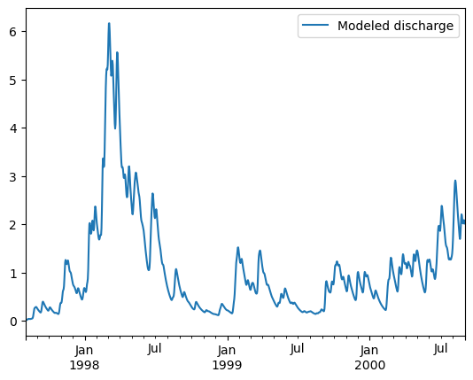
16 In:
df = pd.DataFrame(data=Q_m,columns=["Modeled discharge"],index=time)
17 In:
fig, ax = plt.subplots(1,1)
df.plot(ax=ax,label="Modeled discharge HBV-bmi")
ax.legend(bbox_to_anchor=(1,1));
Using Local HBV model in eWaterCycle
eWaterCycle uses Docker containters to ensure the user has no issues with versioning. When model.initialize(..) is called, in the background a docker containter is started up. This has many benefits for interoperability, but can be slow down a small model like HBV. For this reason, we can use a local model. the first few steps are the same thus these are not repeated. We do need the bmi model locally in the form of a python package.
pip install HBV
Setting up the Local model
We then import the HBVLocal model through the eWaterCycle package:
19 In:
from ewatercycle_HBV.model import HBVLocal
20 In:
model = HBVLocal(forcing=camels_forcing)
21 In:
config_file, _ = model.setup(
            parameters=','.join([str(p) for p in par_0]),
            initial_storage=','.join([str(s) for s in s_0]),
           )
22 In:
model.initialize(config_file)
Running model
23 In:
Q_m = []
time = []
while model.time < model.end_time:
    model.update()
    Q_m.append(model.get_value("Q"))
    time.append(pd.Timestamp(model.time_as_datetime.date()))
After running the model: finalize to shut everything down
24 In:
model.finalize()
Process results
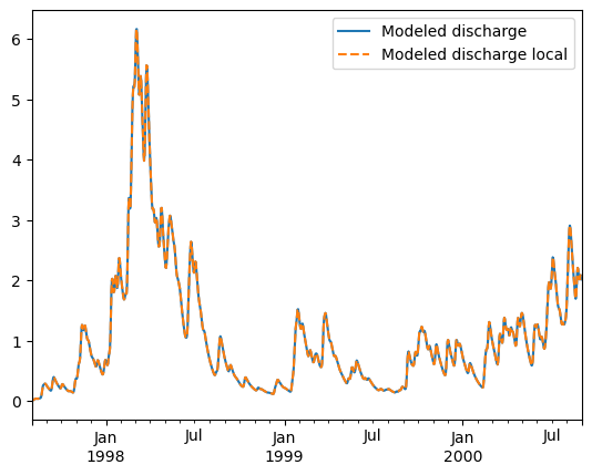
We see these yield the same results, but if we time it: the local model is much faster.
32 In:
df_local = pd.DataFrame(data=Q_m,columns=["Modeled discharge local"],index=time)
33 In:
fig, ax = plt.subplots(1,1)
df.plot(ax=ax)
df_local.plot(ax=ax,ls="--")
ax.legend(bbox_to_anchor=(1,1));